Mark III Systems Blog

In this two part series, I am going to discuss what I consider to be two of the most important hyperparameters that are set when training convolutional neural networks (CNNs) for image classification or object detection.  These are learning rate and batch size.  In this first part, I will discuss learning rate.

Basic Overview of Convolutional Neural Networks

Let's start with a very basic overview of how CNNs work. When training a CNN for image classification, a labeled image is used as input for the neural network.  A lot of processing is done on this input in multiple layers, such as performing convolutions using kernels of different sizes, passing values through activation functions like ReLu, pooling values to downsize the data, and ultimately, classifying the input image into a category.  The image below shows the architecture of the famous AlexNet CNN.

[caption id="attachment_2208" align="alignnone" width="1297"]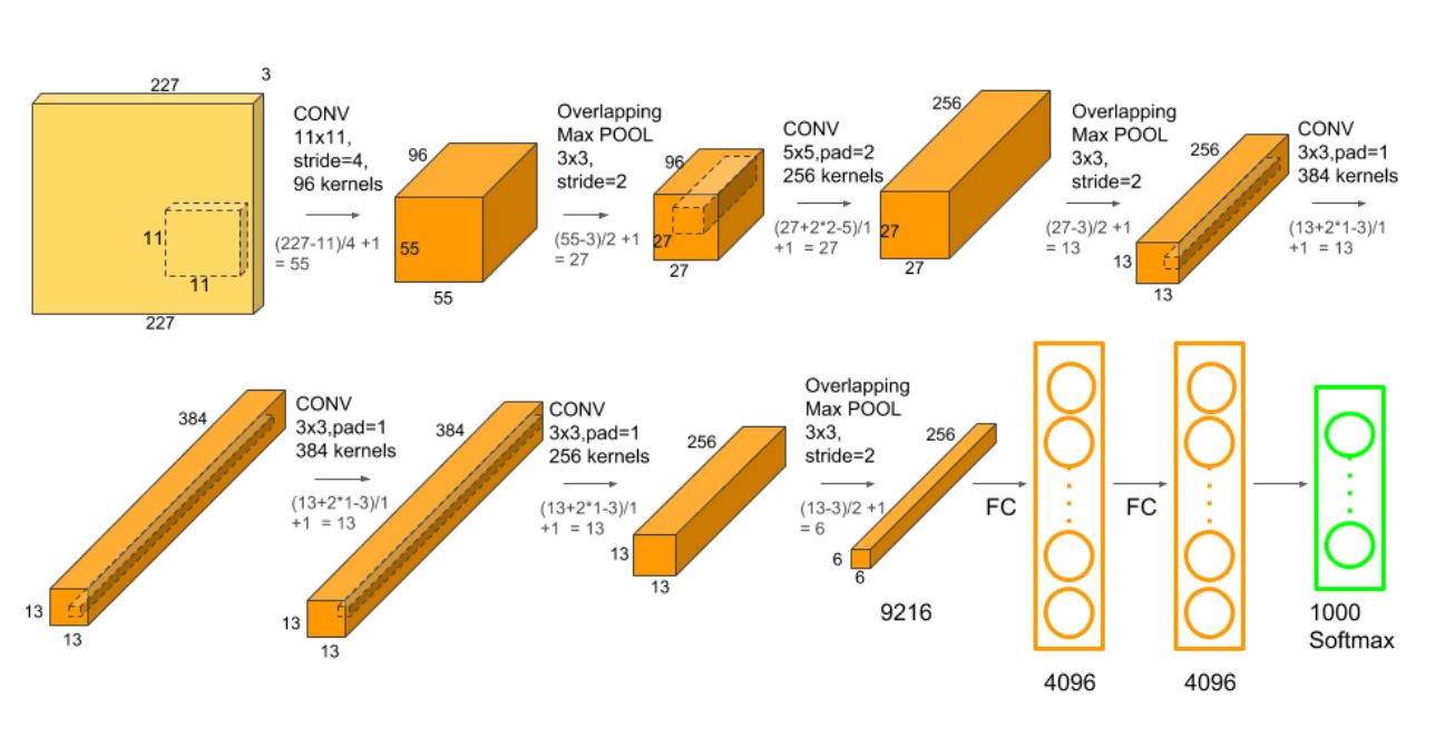 AlexNet (Image from https://neurohive.io/en/popular-networks/alexnet-imagenet-classification-with-deep-convolutional-neural-networks/)[/caption]

The goal during training is to have the network learn the correct weights and biases (parameters) to optimize how well the network classifies images.  When an image is classified in the last layer of the network, one of two outcomes is possible.  It can be classified correctly or incorrectly.  A loss function, sometimes called a cost function, is used to calculate a value known as the loss.  Typically, the lower the loss, the better the performance.  The goal is to optimize the network so the loss is as low as possible without overfitting.  There are many types of loss functions, with cross entropy being one of the most common.

Neural networks use a process called back propagation to update the weights and biases of the network in order to minimize the loss.  The math behind how back prop works is beyond this post, but Matt Mazur (@mhmazur) has an excellent article that clearly explains it.  Learning rate is a critical part of back prop.  If the learning rate is too high, the weights and biases will be adjusted significantly on each pass.  If the learning rate is too low, the adjustments will be very small.  Either of these can cause the network to never converge.  The art is to find a learning rate that will minimize the loss.

A couple of tips to help you find the best learning rate

First, you can either use a constant learning rate, or you can decrease the learning rate over time.  This is known as decay.  For example, for the first 10 epochs, you may use 0.001 for the learning rate.  At epoch 11, you drop the learning rate to 0.0001.  At epoch 20, it drops to 0.00001.  The reason for having the learning rate drop over time is so the adjustments to the  weights become less variable as the network learns.  It's like getting a haircut.  The barber first cuts off long lengths of hair.  Then they make some adjustments and cut shorter lengths.  Finally, they make very small cuts around your ears for the final polishing.  This is exactly what happens when the learning rate drops after a period of time.  I recommend using decay.

Second, start with a high learning rate, say 0.1, or a low learning rate, such as 1e-7.  Learning rates tend to vary from 0.1 to 1e-7, although the large and small ends of that range are much less common.  You will most likely find that these do not work well and may give errors very early in training.  In your next set of experiments, set the learning rate to 0.01, then try again with 1e-6.  Keep working towards a value near the middle and compare the results of each experiment.  You can also start with a middle value, say 0.001 or 0.00001 and work toward the upper and lower numbers in the range.

Once you have trained your network using different learning rates, evaluate the results.  At which learning rate was the accuracy best?  This is typically the learning rate you want to use.  However, learning rate is not the only hyperparameter that makes a difference in model performance.  Next time we will discuss batch size which must also be adjusted to find the optimal value.

Examples of the effect on learning rate on results

Here are the results from some image classification experiments I conducted using Nvidia's DIGITS software running on an Nvidia DGX-1.  The training images (see below for some examples) were letters from tombstones.  There were 10 different letters to classify - A, B, C, E, H, N, O, R, S, and T, and a total of 700 images for each letter.  75% of the images were used for training, 25% were used for validation.  In each experiment, the learning rate was changed and decay was used to lower the learning rate by 1/10th every 10th epoch.

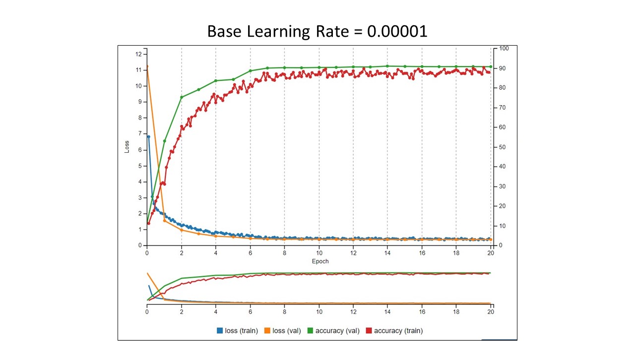
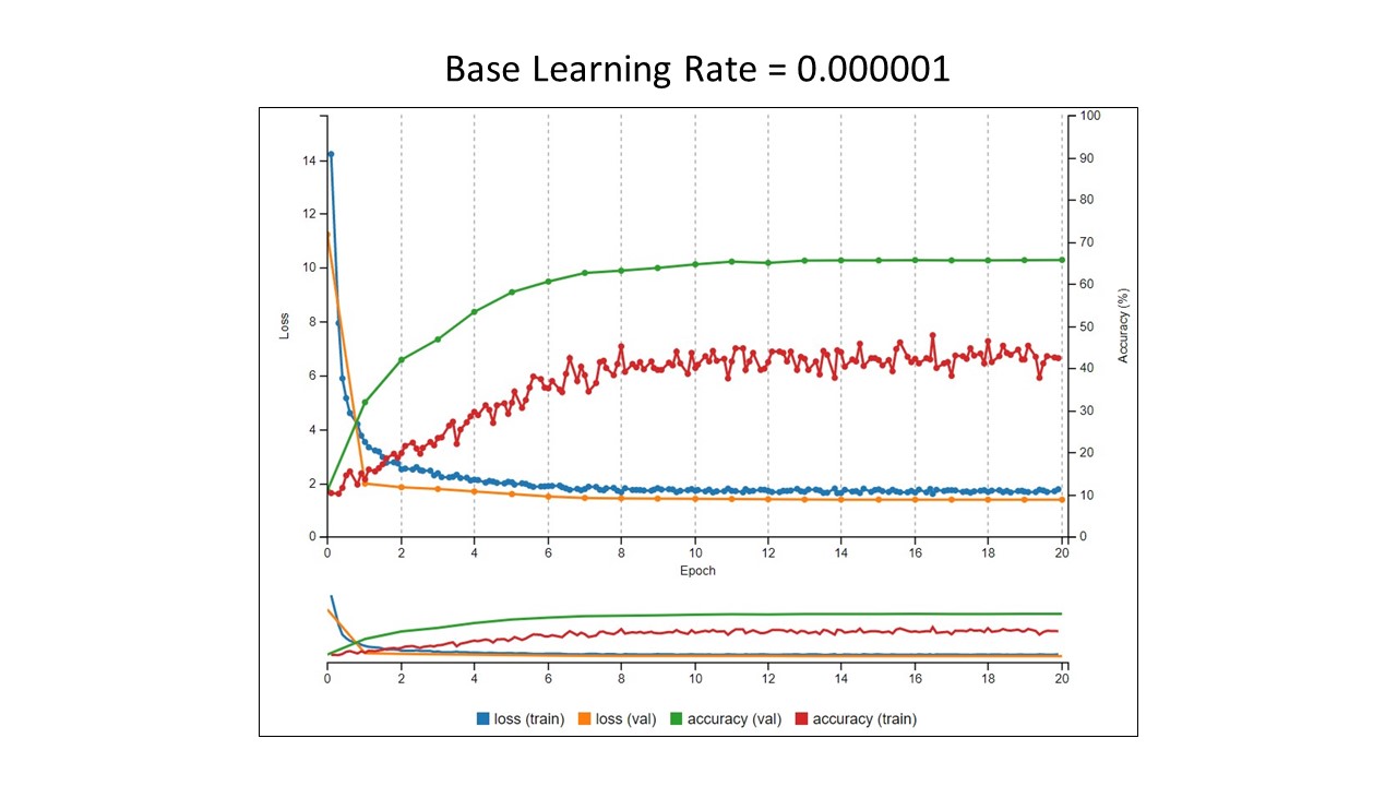
In each Tensorboard image below, the two things to look at are the training loss values in blue and training accuracy values in red. Yes, I know there is more to it than that when evaluating how a model is performing, but for illustration, this is enough. The batch size was 1 in each experiment.  We want to see the loss go down and the accuracy to go up.

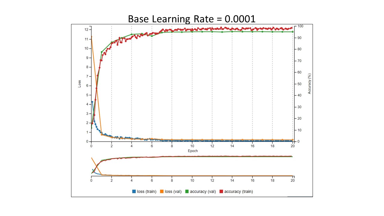
Summary of the results

• We can see that at learning rate values greater than 0.0001, the training failed to converge.  These learning rates will not work.
• At a learning rate of 0.0001, we got a training accuracy of ~95%.
• At learning rates less than 0.0001, the training accuracy decreased.

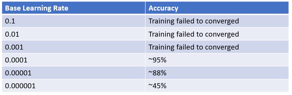From this very simple analysis, we would say that a learning rate of 0.0001 is the best choice for training our model on this data set.  Does this mean this is the learning rate we should use with every data set?  No.  Remember, there is no magical formula. It takes trial and error.  With this set of images in these experiments, this just happened to be the optimal value. Stay tuned for the next installment where I will show how changing the batch size affected the results.