Mark III Systems Blog

Note:

This guide is meant to act as a starting point for someone looking to run ML/DL experiments in the Domino Data Lab framework, an Enterprise MLOps platform. This is a very basic example and assumes that you already have ML/DL experience. This is not meant to be a ML/DL tutorial. This tutorial will also be subject to change as I get more experience with the platform.

Introduction

In this guide I will be illustrating how to run basic ML/DL experiments using the Kaggle Titanic dataset (using NVIDIA A100 GPUs). Essentially we will be using various data points about passengers on the Titanic to predict if they survived or died in the shipwreck. The dataset and associated competition can be found here (https://www.kaggle.com/c/titanic/overview). However, the point is not to get high accuracy in this challenge but to demonstrate a good starting workflow on Domino. Before continuing on, please visit the linked Kaggle competition and download the Titanic dataset provided. 

Dataset

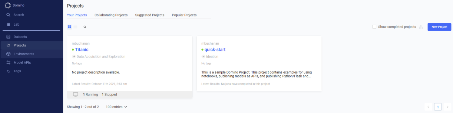
We are going to start by making a project in Domino which will automatically generate a Dataset for us to upload our data up to. To do this, you will want to find the Projects page in the left blue tab as shown in the screenshot below. Click the blue New Project button in the top right corner.

Enter “Titanic” in the Project Name field. Keep the Private mode selected under Project Visibility. Then select the green Create button. 

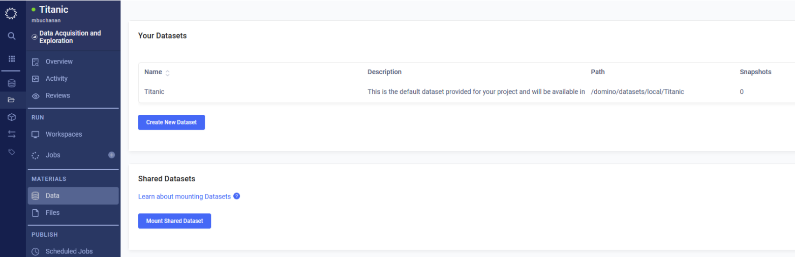
Now we are ready to upload our data to our dataset in our newly created project. Find the Data tab under MATERIALS in the blue left sidebar. Click on Titanic under the Your Datasets section as seen in the screenshot below.

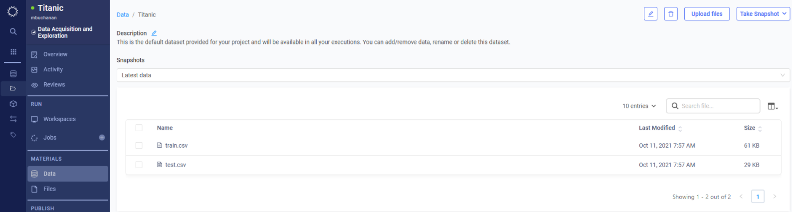
Find the Upload Files button in the top right corner and upload the train.csv and test.csv files which you downloaded from Kaggle in the Introduction section of this document. Your Dataset should look like the screenshot below when you are done.

Now we are ready for data preprocessing.

Data Preprocessing

We need to do some preprocessing on the data we uploaded to our dataset in order to use it in a XGBoost model. We are going to use a Workspace to write some code to manipulate our data. Go to the blue tab on the left and click on Workspaces under RUN.

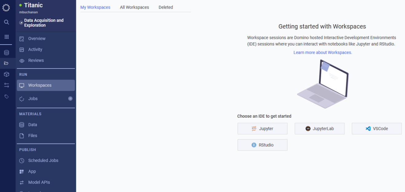
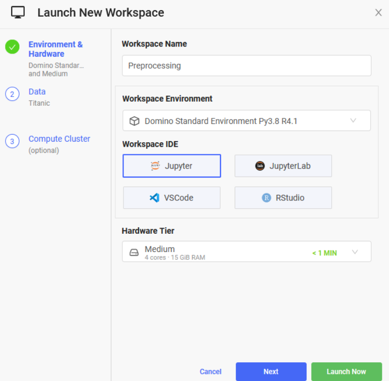
Your screen should look like the screenshot above. Click on the Jupyter button under “Choose an IDE to get Started” but take note of all the options available for Workspaces in case you would prefer a different IDE for your own projects. You should see a popup like the screenshot below. Enter “Preprocessing” in the Workspace Name field. Keep the Workspace Environment set to the default setting and change Hardware Tier to Medium. Notice how our Titanic dataset is already selected in the Data section in the left tab. Then click the green Launch Now button in the bottom right corner.

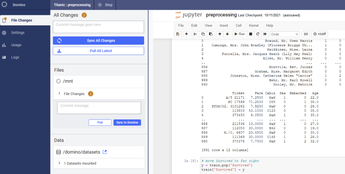
You may need to wait a minute or two for the Workspace to fully load after clicking the Launch Now button. Then you should land on a Jupyter notebook home page. You are then going to want to clone this GitHub repository (https://github.com/michaelabuchanan/domino_guide). Click on the Upload button towards the top right corner and select the preprocessing.ipynb file from the GitHub repository you just cloned. Click on the file after it’s done uploading and a Jupyter Notebook instance should start for you. Select Cell on the top toolbar and click “Run All”. This preprocessing file is extremely basic and essentially only does the bare minimum to get this data to run in our XGBoost model. I would recommend doing much more involved preprocessing for any actual projects you may undertake. Pay attention to the last cell as it shows how to save a file back to the dataset we created in Domino. Also note that in order to see the notebook files we have created in our workspace in the Files section in the Titanic project, not just in the workspace, you need to click on File Changes in the left-most toolbar and then click Sync All Changes as shown in the screenshot below.

Once all the cells in this notebook have run, you should have a new version of the dataset ready to train with. Go ahead and click the Stop button on the top left and then click Stop My Workspace if you get a popup. Then click the Back to Domino button.

Training

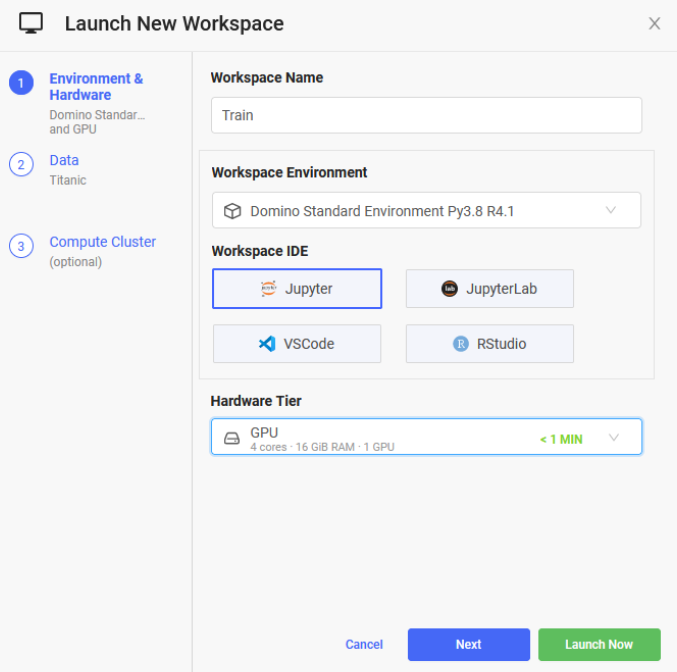
We are going to create a new Workspace in order to utilize GPUs in our training. Click the Create New Workspace button in the top right corner. Enter Train for the Workspace Name and select GPU in the Hardware Tier dropdown. Your screen should look like the screenshot below. Then click the Launch Now button. Once again, it may take a few minutes for the workspace to initialize. 

Now we are going to upload our training Jupyter Notebook. This is going to be the same procedure we used to upload the preprocessing file earlier. Click the Upload button in the top right corner and select the train.ipynb file from the GitHub repository you cloned earlier. Go ahead and run all the cells in the notebook and you should see an XGBoost model train and receive an accuracy score of ~75-85%. This method of training models in Domino is adequate for development but if you want to run training over and over again you will want to switch to running training using Domino’s Jobs feature. We will go over how to do that next, but first go ahead and hit the Stop button in the top left. It is always best practice to stop your environments when you are done using them so the compute resources you were using are available to other users.

Running Training as Jobs

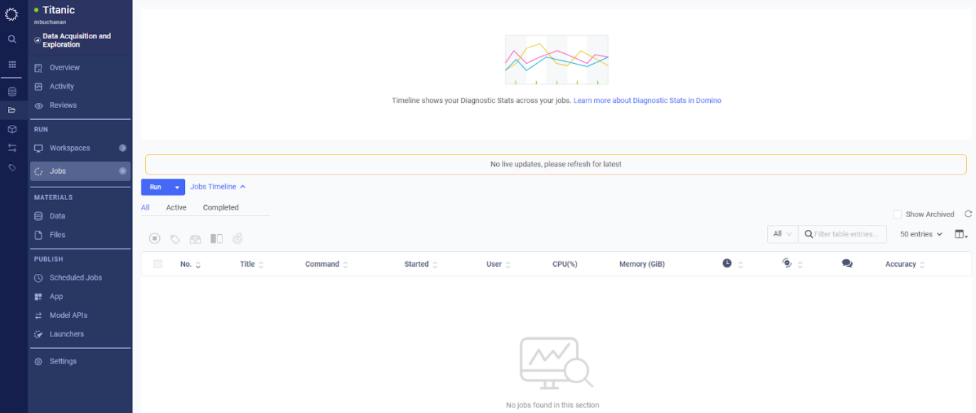
While running training or other scripts in your workspace is a suitable approach for development, it can be beneficial to set up runs as jobs when your scripts are finalized. This can make it easier to experiment with different hyperparameters and easily compare the results. Let’s first look at the Jobs page by clicking Jobs in the left blue toolbar. The page you end up on should look like the screenshot below.

We will be using a slight variation of our training Jupyter Notebook for running our training jobs. Navigate to the Files section in the left toolbar and click the Upload button on the top right. Upload the train.py and dominostats.json files from the GitHub repository you cloned at the beginning of this tutorial. Once that is complete, click on the train.py entry that should now have appeared to view the file. Note that we are looking for a command line argument on line 9. We will be passing different learning rates to this script as we run our jobs to demonstrate how you can experiment with different hyperparameters using Domino jobs. Also note the addition of lines 23 and 24. In order to show the results of our scripts on the Jobs page we need to write the values we would like to display to dominostats.json. In this case we are writing the learning rate and accuracy into this file which means we will be able to see these values for each run of the script we do.

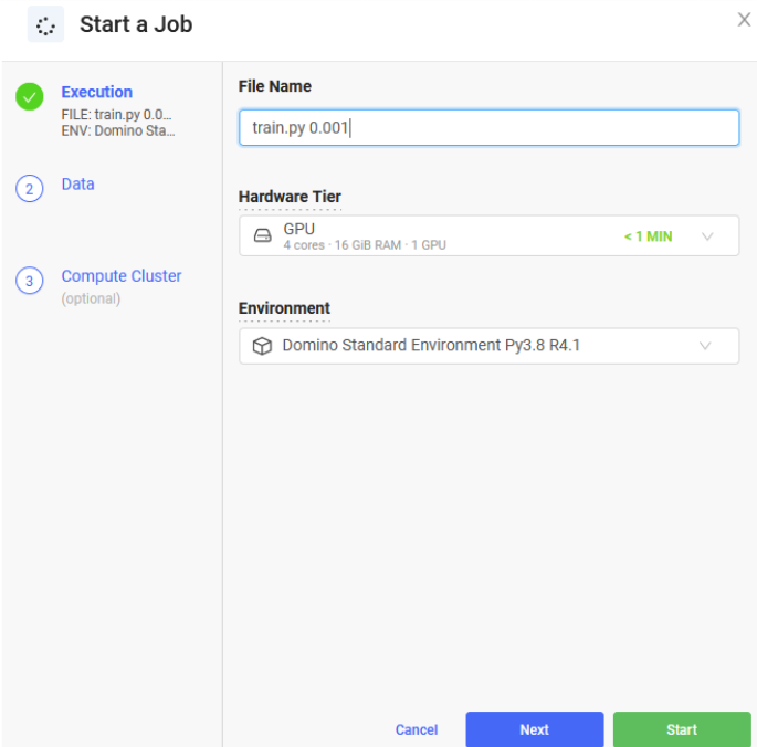
Return to the Jobs page and click the Run button in the top left corner. Enter “train.py 0.001” in the File Name field. The 0.001 is the learning rate we are passing to our script. Feel free to use a different learning rate if you would like. Select GPU as the Hardware Tier and leave all the other settings as they are. Your screen should look like the screenshot below.

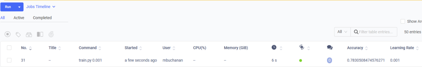
Click the green Start button in the bottom right corner. It will take a minute or two for the job to run. Watch the colored dot to see what the status of the job is. Once it turns green you should see entries in the Accuracy and Learning Rate columns like the screenshot below.

Feel free to play around with running more jobs with different learning rates to see how it affects the resulting accuracy. This concludes this tutorial on basic Domino functionality. Feel free to reach out to me or anyone else at Mark III Systems with any questions or feedback.