Mark III Systems Blog

Over the past few weeks, I have been doing some benchmark testing between the IBM POWER9 AC922 server and the Nvidia DGX-1 server using time series data. The AC922 is IBM's Power processor-based server that is optimized for machine and deep learning. Nvidia's DGX-1 is Nvidia's Intel processor-based server that is optimized for machine and deep learning. Both servers have the latest Nvidia V100 GPU. The AC922 has 2x 16GB V100 GPUs, the DGX-1 has 8x 32GB. This post summarizes the general process used in the benchmarking as well as the results. I have intentionally kept the post somewhat conceptual to illustrate our methodology and key discoveries at a high level. If you want more technical detail, please contact me (john.pace@markiiisys.com).

I chose time series data for the benchmark testing for 2 reasons. First, it is something our customers are asking about. Second, time series problems can be investigated using both classical machine learning algorithms like ARIMA, as well as by deep learning using recurrent neural networks, particularly LSTMs. ARIMA runs solely on the CPU whereas training for LSTMs takes place on a GPU. Thus, this testing allowed comparisons of both CPU- and GPU- based processes on both servers. In addition, it allowed me to compare the relative quality of the predictions made by two very distinct techniques.

In this work, I used synthetic data generated using software by Jinyu Xie called Simglucose v0.2.1, "a Type-1 Diabetes simulator implemented in Python for Reinforcement Learning purpose." Predicting blood glucose levels for patients with diabetes is of particular importance because the models can be used in insulin pumps to predict the correct amount of insulin to give to normalize blood glucose levels. The software generates synthetic blood glucose data for children, adolescents, and adults at designated time points. I used data at 1 hour time points. The training data consisted of 2,160 time points (90 days). The prediction data consisted of 336 time points (14 days). So, the models were trained using the 90 days of hourly time points, then tried to predict the hourly values for the next 14 days.

Two different algorithms were used to make the predictions. The first was a classical machine learning technique known as ARIMA (Autoregressive Integrated Moving Average), more specifically, SARIMA (Seasonal Autoregressive Integrated Moving Average). SARIMA is a specialized version of ARIMA that takes into account seasonality of the data (blood glucose levels have a very clear seasonal pattern). The second was an implementation of a recurrent neural network known as an LSTM (Long Short-Term Memory). To perform the comparisons, I used Jupyter notebooks that ran Python scripts. Thanks to Jason Brownlee of Machine Learning Mastery for his publicly available code that was adapted for this project. I compared the predictions for the SARIMA and LSTMs using Mean Squared Error as the quantitative metric of how well the model made predictions. I also calculated the time it took for the training and predictions to be done. For SARIMA, I only calculated the total run time for the training/prediction calculations since there is no distinct prediction phase. For the LSTM, I calculated separate run times for the training and prediction phases since they are distinct processes.

For training and predictions, I used synthetic data for adolescents that I termed as Patients 001, 002, 003, 004, and 005. For each patient, the 2,160 hourly training data points and 336 prediction data points were generated. I then did pairwise comparisons of all patients. For example, I would train a model using the training data for patient 001. I would then use that model to make predictions for patients 001, 002, 003, 004, and 005. The process was repeated for all patients. This gave a total of 25 comparisons. Full pairwise comparisons were performed to evaluate if either SARIMA or LSTM could create models that could be generalized to other patients.

Not surprisingly, the models could not be generalized, which was the expected result. This result underscores the importance of using relevant data to train machine learning models.

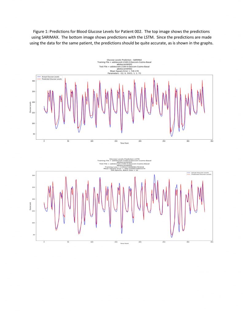
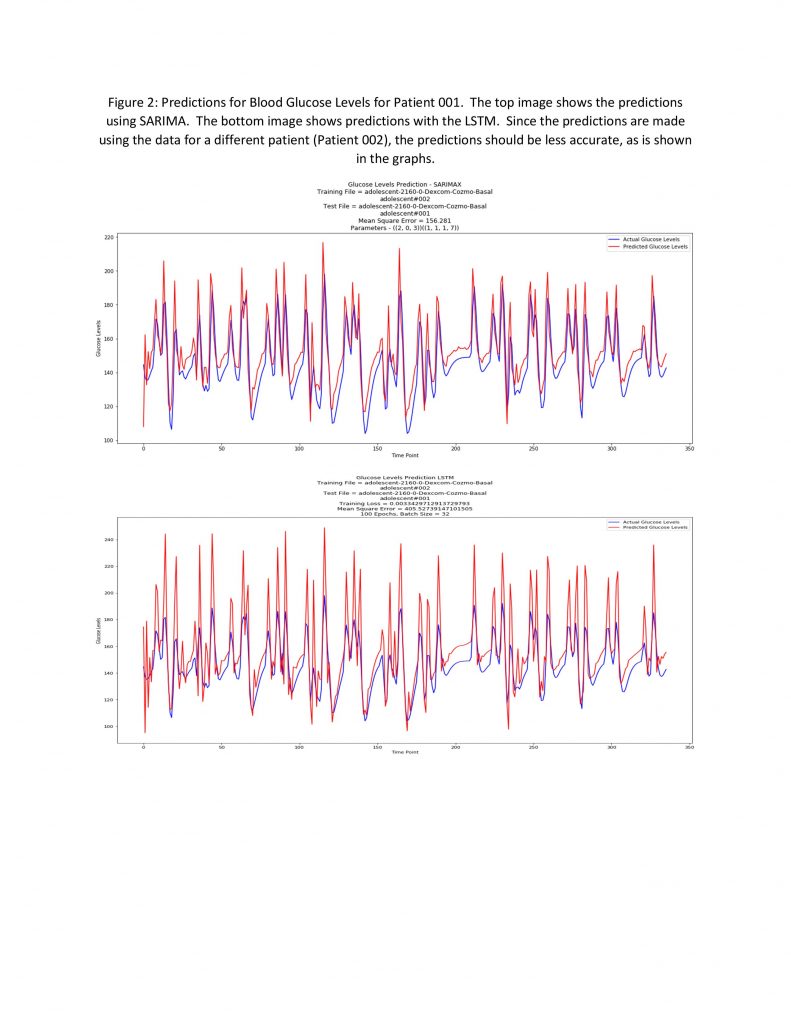
Below are examples of how the models performed on predictions. The blue lines are the actual values and the red lines are the predicted values. In the first 2 images, the model was trained on the data for Patient 002. Predictions were then made for Patient 002. In the last 2 images, the model was again trained on the data for Patient 002. Predictions were then made for Patient 001. As you can see, the results were significantly less accurate than when values for Patient 002 were predicted.

The results I obtained were very interesting. Here is a very high-level overview.

• For the SARIMA training and predictions, which run strictly on the CPU, the DGX-1 performed an average of 42.9% faster than the AC922 (range 29-48% per patient).
• For the LSTM training phase, which runs strictly on the GPU, the DGX-1 performed 8.0% faster than the AC922 (range 6-11% per patient).
• For the LSTM inference phase, which runs strictly on the CPU, the AC922 performed 16.9% faster than the DGX-1 (range 8-28% per patient).
• The total training/prediction time for SARIMA was several orders of magnitude faster than training and prediction using LSTM. The average total training/prediction time for SARIMA on the DGX-1 was 7.7 seconds and 13.8 seconds on the AC922. However, the average LSTM training/prediction time on the DGX-1 was 2,478.1 seconds (321.8 times slower than SARIMA) and 2,693.7 seconds on the AC922 (179.6 times slower than SARIMA).
• In some cases, the MSE for SARIMA was lower than for LSTM and vice versa, so it is difficult to say which model actually performed better in making predictions. In all cases, the MSE for the SARIMA and the LSTM were comparable with each other (see images above). This outcome could vary significantly based upon how the LSTM network is built and how the hyperparameters for the SARIMA model are chosen. For these benchmarks, the goal was not to find optimum hyperparameters, but rather to evaluate the performance of one server versus the other on identical machine learning/deep learning tasks.

So, the burning question is, "Which server is better for time series analysis? The Nvidia DGX-1 or the IBM POWER9 AC922?" The answer is both. For SARIMA and LSTM training, the DGX-1 outperformed the AC922. For LSTM predictions, the AC922 outperformed the DGX-1. Which one should you choose? The answer depends on the use case. If you want to use SARIMA or if LSTM training time is your driving factor, the DGX-1 may be the better choice. If prediction speed is critical, the AC922 could be better.

Admittedly, there are a couple of caveats that must be considered. There were some version differences of pandas, NumPy, TensorFlow, and Keras due to the differing processor architectures. I tried multiple versions of each and the results were very similar. Also, the DGX-1 uses Docker containers while the AC922 uses conda environments. This could lead to some differences as well. Overall, I think these differences have very little effect on the overall benchmark outcomes, but it is something I plan to investigate further. Finally, the models were trained on a small dataset, only 2,160 data points. I will be trying a much larger dataset in the future as well as trying different combinations of hyperparameters to improve forecast accuracy.

The Jupyter notebooks, scripts, and data files, along with all of the summary statistics are available on my GitHub page.

Citations:

• Brownlee, Jason. 11 Classical Time Series Forecasting Methods in Python (Cheat Sheet). (January 9, 2017) [Online]. Available:
  https://machinelearningmastery.com/time-series-forecasting-methods-in-python-cheat-sheet/ (Accessed 2019)
• Brownlee, Jason. How to Develop LSTM Models for Time Series Forecasting. (November 14, 2018) [Online]. Available: https://machinelearningmastery.com/how-to-develop-lstm-models-for-time-series-forecasting/ (Accessed 2019)
• Jinyu Xie. Simglucose v0.2.1 (2018) [Online]. Available: https://github.com/jxx123/simglucose. (Accessed 2019).